RAM-AI
Tel. +41 58 726 87 00
E-mail contact@ram-ai.com
Contact UsRAM’s
Machine learning
Artificial intelligence (“AI”) has arguably become the most significant and disruptive general purpose technology in recent years.
Techniques like machine learning (“ML”) have taken giant strides forward; empowering computers and enabling them to learn and build models so that they can perform prediction across different domains.
This technology is particularly pertinent to the portfolio management industry, where the integration of information from numerous, large – and often unstructured – datasets has become a key success factor.
ML development frameworks accessible to the research community now offer solutions to both handle these datasets and interpret results, controlling how inferences are derived. We believe that what we teach the machine is only as important as the limits and constraints we set during its learning process, unlocking interpretability and generalization.
In this paper we will look at the growing popularity of artificial intelligence and the potential for finance to prosper from machine learning implementations. As technology continues to push the boundaries of our imagination, new dimensions will undoubtedly emerge over time.
Machine Learning
1950’s
Artificial
Intelligence
From a
concept ...
1980’s
Machine
Learning
To a set of
predictive techniques
2000’s
Deep
Learning
Learning in always more levels of abstraction
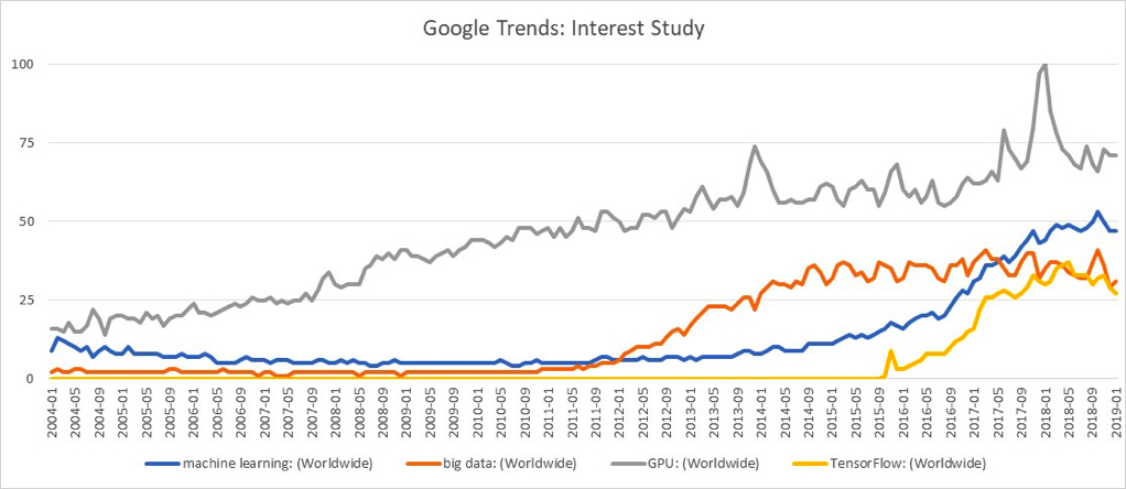
Web-search data from Google Trends provides an interesting insight into what’s driving the recent enthusiasm for machine learning techniques:
PART 1
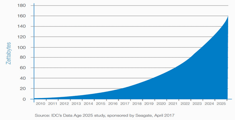
Digital data has seen exponential growth since the early 2000s. This growth has occurred across both structured data (highly organized contents such as relational da- tabases) and, more importantly, unstructured data (such as emails, files, etc.). Unstructured data now represents roughly 80% of the total data but is harder to analyze. Most of this data is generated automatically by mobile devices and computers (e.g. social network platforms) but also by sensors; a modern car has more than 100 sensors!
The International Data Corporation (IDC) forecasts that by 2025 the global datasphere will grow to 163 zettabytes (i.e. 163 trillion gigabytes)1. The amount of data gene- rated every day should be around 50 billion gigabytes, which is ten times the amount created between the dawn of civilization and 2003 – this amount was estimated at around 5 billion gigabytes by Hal Varian, Chief Economist at Google.
Data Created Over Time
As investor focus has turned to higher frequency and alternative data sources, financial data has witnessed tremendous growth, enabling investors to take more in- formed decisions. In addition to traditional data sources (market prices, volumes, financial statements, analysts’ estimates, etc.), investors now have access to a wider range of alternative datasets enabling far greater insight. This alternative data comes in the form of more-or-less- structured datasets such as ESG indicators, management transactions, sentiment-driven data based on newsfeed and social media, earnings call transcripts, web-searches and web-traffic data, credit card, and – generally unstruc- tured – sensor data records (e.g. geo-location, satellite, weather, etc.).
Number of alternative datasets by launch date
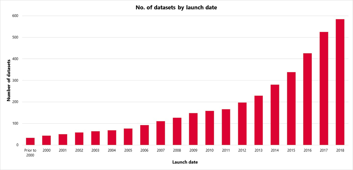
Source: Neudata & RAM Active Investments
1Reference: https://www.seagate.com/files/www-content/our-story/trends/files/Seagate-WP-DataAge2025-March-2017.pdf
PART 2
The research community now has access to significant processing power …
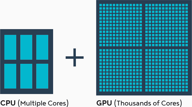
The machine learning boom has benefited from the steady cheapening of hardware and developments achieved in recent years – sometimes to serve other purposes. Graphics Processing Units (GPUs), which were originally designed for rendering graphics for game players, can now be used for general purpose calculations, just like Central Processing Units (CPUs). This has helped to dramatically accelerate the training of machine learning algorithms. Indeed, modern GPUs contain thousands of processing cores, many more than CPUs; allowing them to execute thousands of operations in parallel during one clock cycle. However, GPUs generally run at a lower clock speed than CPUs. For example, the NVIDIA GTX 1080Ti 11GB Graphics Controller contains 3’584 physical cores and 12bn transistors, whereas the Core Intel i9-7900X 3.3GHz processor has 10 physical cores and probably a few billion transistors, (although this number is undisclosed). Title: At the core: CPU vs GPU
At the core: CPU vs GPU
The number of transistors on an integrated circuit (transistor count) continues to grow at a pace, albeit slightly slower than Moore’s law (according to which it should double approximately every two or two and a half years). These transistors are used both in processing and storage units. The chart below illustrates the number of transistors per processor.
Number of Transistors per CPU / GPU
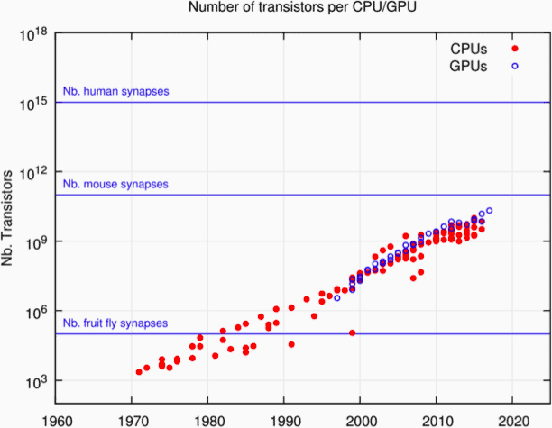
The number of transistors in modern processing units is fast approaching the number of synapses in a mouse’s brain !
“ Every 5 years, computers are getting 10 times cheaper ! ”
Schmidhuber
Similarly, the storage capacity of the various randomaccess memory (RAM) modules – used to store input data, temporary data, weights and activation parameters of ML algorithms – has increased steadily. These modules are essential in optimizing computing power: SRAM (Static RAM) is a low-density, fast storage solution which is generally embedded within processing units in order to feed them with the immediate data they need, while cheaper/ slower DRAM (Dynamic RAM) are used as main memory to store less immediate data used in ML algorithms. These have also cheapened significantly!
… And both hardware and cloud providers have joined the race!
GPU usage has been made possible through specific Application Programming Interfaces (APIs). APIs are a software intermediary that allows two applications to talk to one another. NVIDIA was the first GPU maker to propose their proprietary API called CUDA. NIVIDIA have taken a quasi-monopoly (for now) – on the general-purpose GPU acceleration market. NIVIDIA’s dominant position has even enabled them to change the terms of their software licensing agreements. This change prohibits the use of consumer-grade (GeForce) cards by firms in data centers, forcing firms to utilize the more expensive institutional-grade (Tesla) cards. In parallel, the world’s major players of cloud computing (Google, Amazon and Microsoft) have seemingly joined a race towards offering ever-greater processing power on their cloud platforms –ensuring they stay current - to rival the best GPU infrastructures. Google was the first to provide access to NVIDIA’s GPUs (P100), but Amazon responded by offering access to the more powerful Tesla Volta GPUs (V100-backed P3 instances that include up to eight GPUs connected by NVLink).
Google’s Cloud TPU2

In February 2018, Google offered access to Tensor Processing Units (TPUs) through their cloud platform. TPUs are a form of application-specific integrated circuit (ASIC). Google designed these units specifically to optimize the use of their ML development framework, TensorFlow, and enabled the use of Compute Engine virtual machines to combine the processing power of several units. While Google’s first-generation TPUs were designed to run only pre-trained ML models, their second-generation Cloud TPUs are more powerful and designed to accelerate both the training and the running of ML models. Each v2 TPU provides 180 teraflops (floating-point operations per second) of ML acceleration, which is the equivalent of 15 consumer-grade graphic cards such as the NVIDIA GTX 1080Ti. The latest water cooled V3 TPUs reach 420 teraflops, are equivalent to the recent NVidia DGX-Station (which delivers 500 teraflops for a purchase price of roughly $50’000).
PART 3
The bright outlook for AI applications has encouraged large tech corporations like Google, Facebook, Amazon and Microsoft to invest heavily in the field of machine learning. These names have committed resources to create ML development frameworks for their own needs but have also been enthusiastic in releasing them “open-source” to the research community. Popular ML frameworks include; PyTorch (released by Facebook in early 2017), TensorFlow (open-sourced by Google Brain in 2015) and MXNet (main backers being Amazon and Microsoft). These names have certainly contributed in developing a collaborative and active community, made up of researchers, practitioners and machine learning enthusiasts, and to the popularity of data science competition platforms like Kaggle.
These frameworks consist of a high-level interpreted language and are built upon a fast and low-level compiled backend to access computation devices including GPUs. They also generally offer data input/output solutions and convenient ways of modelling the building blocks of the network, commonly called “tensors”, as well as performing operations on them; tensors are used to encode the signal to process, but also the internal states and parameters of the ML algorithms.
There are multiple reasons behind this open-sourcing by these tech giants; they obviously see an opportunity to lure more talent to help improve these frameworks (or simply recruit them), and to try to become an industry standard within the research community to benefit from various applications. But they possibly intend to profit from their dominant position regarding data and processing power – and the clear oligopoly here – to control all the technology surrounding ML.

Machine Learning
PART A
Machine Learning has often been defined as a “field of study that gives computers the ability to learn without being explicitly programmed” (Arthur Samuel, 1959). The general objective of ML is to capture regularity in data in order to make inferences or recognize certain patterns.
Indeed, many applications such as image recognition and language translation require the automatic extraction of “refined” information from raw signals.
In the context of finance, most references to AI techniques general concern a predictive ML model; the terms Machine Learning and Artificial Intelligence are often used interchangeably and stand for a collection of statistical techniques ranging from ordinary least squares regression to Neural Networks and Deep Learning.
PART B
Machine learning can be reduced to two primary categories; supervised and unsupervised learning. The objective of both approaches is to make inferences from input variables, however:
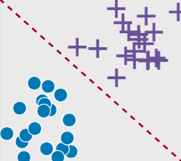
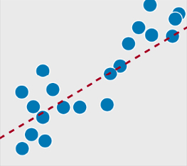
Supervised learning seeks to map these input variables to an output variable; thus it requires training data to be labelled, i.e. to have, in addition to other features, a parameter of interest that can serve as the “correct” answer. Supervised learning is well-suited to:
Classification problems
(when the labels are discrete):
Classification
Regression problems
(when the labels are continuous):
Regression
Unsupervised learning seeks to describe the structure of unlabeled data. It is called “unsupervised” as there are no correct answers and no supervisor (teacher). For example:

Netflix’s market segmentation through clustering instead of geographic, is to discover the inherent groupings in the data. Netflix observed that geography, gender, age and other demographics are not significantly indicative of the content a given user might enjoy.

Amazon’s item-to-item collaborative filtering aims at discovering association rules that describes large portions of input data, such as customers who buy a given product may also tend to buy another related product.

Google’s PageRank algorithm based on network analysis looks to discover the importance and the role of nodes in the network and measure the importance of website pages.
PART C
Unsupervised learning can be applied to dimensionality reduction or feature selection on an input dataset such as the time series of standard or alternative factors across a universe of stocks; to find a smaller set of variables (either a subset of the observed variables or a set of derived variables) that captures the essential variations or patterns.
The process can be dependent on the original learning task when it is known (e.g. predicting stock price, volatility or volume), or not (e.g. auto-encoders as non-linear alternative to PCAs for dimensionality reduction).
Supervised learning can be used for stock selection, the objective being to predict future stocks’ behaviors based on an historical dataset of inefficiencies.
These expected senbehaviors can be either continuous (a function of expected return and risk, for example), or discrete (will a given stock outperform or underperform a given benchmark, etc.).
The recent development of ML frameworks for deep learning models also allows the efficient capturing of patterns in a time series. For example, convolutional neural networks (CNNs) commonly applied to image recognition, can also capture financial time series dynamics.
Similarly, LSTM (long short-term memory) networks and other types of RNN (recurrent neural networks) can help capture events with long-term memory, corresponding to market corrections for example.
PART D
This is similar to biological systems for which the model (e.g. brain structure) is DNA-encoded, and parameters (e.g. synaptic weights) are tuned through experiences.
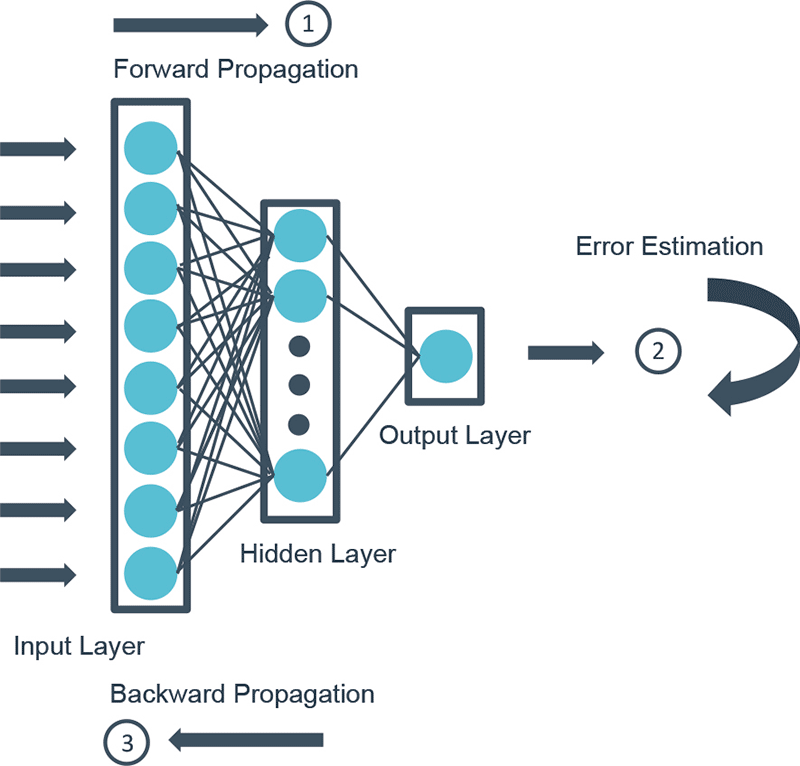
The most common training procedure is the “gradient descent optimization”, which allows to estimate optimal model parameters by performing several training steps.
At each step, the backpropagation reassesses the sensitivity (gradient) of the prediction errors (between predictions and the actual values to predict) to changes in model parameters, in order to update model parameters and help them converge towards an optimum. The size of the shift in model parameters at each step is determined by a hyper-parameter known as the learning rate.
Example
PART D
These models are generally complex and involve an additional set of parameters called hyper-parameters, which contribute to specify the model and define the way it trains:
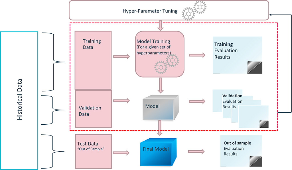
These hyper-parameters are not set during the training procedure; they must be tuned before the training, either manually or by using grid search or Bayesian optimization techniques. The picture below shows a typical calibration process for a ML model, in which its parameters (e.g. neuron weights) are set through training, and its hyper-parameters are set through an iterative process.
At RAM, we believe a robust way of deploying a ML model consists of implementing such an iterative process through a cross-validation technique, which, at each iteration (which corresponds to a full training for a given set of hyperparameters), randomly generates a training sample (sample of data used to fit the model) and an unseen validation sample (sample of data used to provide an unbiased evaluation of the model fit on the training sample).
The presence of a training set and a validation set as well as the potential use of cross-validation techniques to generate them are essential in ensuring the generalization of the model – i.e. detecting potential over-fitting. It is also key to initially isolate a test dataset, aimed at providing an unbiased evaluation of the final model. This is typical of a trial-anderror process, where the system tries to extract regularity from raw input data by performing several feedback loops!
Typical prototyping phase of a ML model
Our Approach
PART A
At RAM, our systematic stock picking methodology seeks to capture persistent inefficiencies across a given universe of stocks. To do so, we need to abstract data from financial datasets such as time series of stocks’ features (“factors”). These factors can be classified as “traditional” (value, low-risk, momentum, quality, etc.) or more “alternative” (ESG indicators*, management transactions, sentiment data from newsfeeds and social media, etc.). High-dimensional data processing allows us to make informed predictions, simultaneously integrating information from across all these factors.

Helps to capture stocks that may not be a pure Value, low-risk, Growth Momentum profile, but are highly alpha generative being great by all standards
In addition to the increasing number of variables, we also have to treat a large amount of data points across several geographical regions, long-term time horizons and various frequencies – some of our datasets have more than 20 years of daily history.
Machine learning models can be seen as a natural generalization of data processing techniques; perfectly adapted to the high dimensionality of our datasets, combined with the flexibility they require:
ML development frameworks are optimized to manipulate tensors, i.e. multi-dimension arrays, and benefit from the high processing power offered by CPUs, GPUs and TPUs (and their high-capacity RAMs).
The optimizers embedded in these frameworks are extremely powerful to train deep learning models, they have been developed specifically to solve multi-dimensional problems (picture recognition, consumer clustering, etc.).
The process of adding new variables to an existing dataset is very easy, and several ML techniques allow quick assess if such variables bring new information to our stock selection process; this is convenient to test the potential added-value of alternative datasets.
Unsupervised machine learning techniques and features selections techniques can also be used to reduce the dimensionality of the problem, if needed.
PART B
The input factors we use are obviously not independent variables. They interact with each other in a way which is a-priori unknown, although these interactions might make intuitive sense. For example, low-quality stocks which have high earnings accruals tend to have inflated earnings, therefore lower price-earnings ratios, which makes them cheaper according to one measure of value.
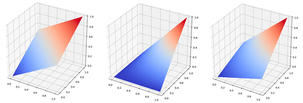
One way of modelling interactions in standard data analysis, such as linear regressions, is to add several first-order interaction terms in the form of products of two variables into the input dataset. For example, charting the preference curve (y) using ranked factors for value (x) and quality (z), we can see that a name with average value and average quality (x=50%, z=50%) will score higher than an extremely cheap name of extremely bad quality (x=100%, z=0).
The aim here is to maximize the preference curve, given high score vs low score on another metric.
Modeling of Interactions Between Value & Quality
Source: RAM Active Investments
However, we can anticipate that these interactions are unlikely to be linear, and that some higher-order interaction terms could be required in some instances. For example, the interactions between leverage (as measured by Debt/Equity) and future returns are clearly not linear: on the one hand too much debt can be a consequence of over-investment and result in high interest costs, (weighing on future returns); on the other, too little debt might dampen growth. There must be an optimal amount of debt somewhere between from these two extremes.
It is obviously difficult to model the structure of dependencies within our input dataset given the high diversity of input factors and non-linear causality relationships.
A copula-based technique (some form of parameterization of the joint cumulative distribution function) could be used to model these interactions, but at the cost of high calibration complexity – and subsequently a high risk of poor generalization.
One of the advantages of ML techniques is that they require almost no assumptions on the structure of interactions. We have observed that random forests and neural networks work well to abstract these dependencies and make predictions: when calibrated accurately, they generally outperform regressions and logistic regressions with first-order interactions terms.
Machine learning techniques also provide non-linear alternatives to standard dimensionality reduction techniques such as PCA (principle component analysis), sometimes used to remove “noise” from input signals. We can use, for example, an unsupervised machine learning technique called auto-encoder (AE); AE also refers to manifold learning. We can illustrate this comparison by using an auto-encoder based on a neural network showing a bottleneck configuration, which seeks to predict the identity function
We can use PCA and AE to reduce the dimensionality of a dataset of more than 200 factors, to a limited number of factors, thus improving the generalization capabilities of a subsequent model. This can prove useful if the model is complex (tends to overfit, e.g. boosted trees) or if input data has many outliers.
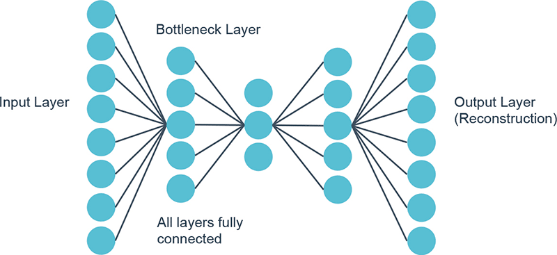
Example
PART C
All data that does not qualify as structured is unstructured, this describes newly created data that hasn’t been (or fully) explored, cleaned and processed. It is usually laden with text but may also include audio and/or visual data. In the context of finance, textual datasets include news, social media, earnings calls transcripts, etc.
“ Various alternative and unstructured datasets are now available to the investment community, and extracting information from them can clearly provide an edge for stock selection strategies. ML frameworks provide tools to structure these datasets and extract semantics from them. ”
At RAM, we are exploring ways to unveil the hidden information in some of these datasets, e.g. to extract the sentiment of an earnings call to enhance a stock selection strategy. ML development frameworks provide powerful techniques to handle these through NLP (Natural Language Processing), i.e. leveraging computing power and statistics to process and clarify language in a systematic and sensible way that doesn’t involve human intervention (besides coding).
There are generally three major steps in NLP: text preprocessing, text to features and testing & refinement. Text preprocessing includes noise removal, lexicon normalization and objective standardization. Text to features includes syntactical parsing, entity parsing, statistical features and word embedding.
Structuring the preprocessed text through word embedding (a method of using a vector of numbers to capture different dimensions of a word) can typically transform it in a set of a few hundred numerical features (dimensions), making subsequent analysis easier!
PART D
The first objective when fitting a ML model must be to ensure that the model is sufficiently robust, i.e. it must generalize well on unseen data. To do so, many techniques can be used in combination: using cross-validation (i.e. isolating various training and validation samples as described previously), using large enough datasets, and using regularization techniques. Regarding cross-validation, it is vital to compare the speed and smoothness of the convergence of the various training and validation datasets, as well as the distribution of model weights throughout the various training iterations; various visualization tools such as Google’s Tensorboard can help. ML frameworks also make it easy to use and compare several regularization techniques. For example, the various optimizers generally embed a weight decay parameter, which allows to implement ridge regularization (i.e. to force the weights to be small without being zero) during the training procedure.
At RAM, one aspect of the application of ML techniques that we believe should not be underestimated is interpretability, i.e. understanding how & why results are generated. Model interpretability aims to help us understand why a machine learning model made a given decision and to gain comfort that the model is correct (and for the right reasons). Model explainability has been an increasing area of research, especially in the last 2 to 3 years, as demonstrated by the many tutorials on model interpretability in the recent flagship conferences on machine learning. In particular, many topics were covered at ICML 2017 (International Conference on Machine Learning) and NIPS 2017 (Neural Information Processing Systems), including sensitivity analysis, mimic models, and investigating hidden layers.
Numerous competing packages to enhance model explainability were presented at these conferences, including SHAP - SHapley Additive exPlanations. SHAP purports to be a unified approach to explain the output of any machine learning model. SHAP connects game theory with local explanations, uniting several previous methods and representing the only possible consistent and locally accurate additive feature attribution method based on expectations.
Our Approach
PART A
At RAM we have been working for over 12 years on building several factors for stock selection, which seek to capture various inefficiencies such as momentum, growth, quality, value, low-risk, etc. Although we have designed every single factor with the view to extract information about a given inefficiency as efficiently as possible, all these factors need to be preprocessed so that our machine learning models can infer accurate predictions from them. Preprocessing is crucial, especially for deep learning models which are using neural networks, for which convergence is clearly helped when data is cleaner. Cleaning the data means working on the distribution of inputs, the potential presence of non-available data, and identifying causes for outliers, in order to potentially retreat them.
Among other techniques, we are using the Scikit-Learn package for these processing steps, in particular their various scalers:
Quantile transformer: Rank transformation in which distances between marginal outliers and inliers are shrunk. Gaussian transformer: Another non-linear transformation in which distances between marginal outliers and inliers are shrunk. Standard Scaler : Removes the mean and scales the data to unit variance. Robust scaler : Removes the median and scales the data according to the quantile range (by default the interquartile range).
PART B
Feature selection
As discussed previously, over the course of the last 12 years, we at RAM have built a repository of numerous fea- tures capturing a variety of market inefficiencies on the back of traditional and alternative data sources. We use deep learning to combine all these stock features when predicting a stock’s return, risk and liquidity dynamics. Deep learning approaches provide us with an optimal non-linear combination of these features, revealing their non-linear interactions.
We face numerous challenges when building a deep learning model combining a multitude of features:
To overcome all these issues, there is a lot to gain by doing a feature selection before training a model when one has a large number (hundreds, thousands or more) inputs.
The feature selection process will first look to identify the most informative and relevant features to predict the output variable. They are the set of variables that should together help predict in the most robust manner the out- put variable.
Univariate feature selection
The simplest way to select input features is to retain those that have the strongest relationship with the output variable. The most basic approach would be to select the features that are most highly correlated with the output variable. To better assess the linear relationship and consider the significance of this correlation, one can use a F-test which estimates the degree of linear dependency between each input and the output variable, selecting the top ranked ones.
But the limit of correlation or F-test scoring is that they only reflect linear relationships between the input and output va- riables, when there are often non-linear interactions at play in our data. In this case it would be more useful to conduct a more general univariate test looking at mutual information between each input and the output variable. Mutual infor- mation being entropy-based, can uncover any statistical dependency to help select the most relevant features.

Linear v Non-Linear Relationships
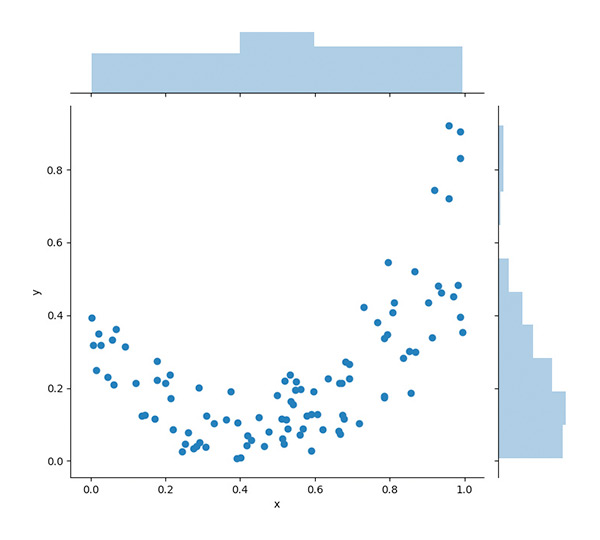
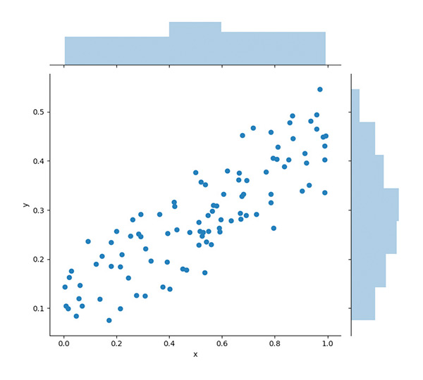
There is, however, a very strong limit to univariate tests to achieve a robust feature selection, as they retain the best features to explain the output on a stand-alone basis but totally ignore the complementarity or the redundancy of the features retained. In practice, the input features often exhibit a significant degree of correlation, making univariate tests sub-optimal.
Linear v Non-Linear Relationships
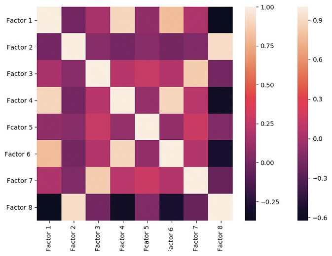
Hence the need for feature selection with a multivariate angle capturing the complementarity of the inputs to identify an overall optimal group of variables.
Regression-based ranking
We can fit a multivariate linear regression model to explainzbr the output variable with all features and rank eachzbr feature along its statistical significance to retain the mostzbr explanatory ones.
The downside in this feature selection approach lies inzbr the fact that a number of highly correlated input factorszbr can still be retained, as often they would tend to havezbr large betas with opposite signs and high statistical significance in a multivariate regression. This subsequently increases the risk of having a sub-optimal set of features in the deep learning model.
Lasso
A feature selection based on a Lasso model can help to overcome the limits of a linear regression by reducing the likelihood of multiple highly correlated features being retained. A Lasso adds a penalty that sums up the absolute scale of the regression betas, a “L1” penalty, which forces many parameters to be zero as the strength of the regularization increases. Weak and redundant features rapidly end up with zero coefficients, making the Lasso well-suited for a robust feature selection.
Recursive feature elimination (RFE)
Recursive feature elimination (RFE) is a process that aims to ensure one misses the least interactions between features, by gradually taking into account how these interactions change as we reduce the size of the feature set.
It starts by fitting a model with all input variables, then iteratively eliminates groups of k variables at each step with the least importance in the model. One typically evaluates the importance of a variable by measuring the reduction of accuracy of the model when it is eliminated.
The model is then fit again with the reduced feature set, to then exclude k variables again, and so on, until we reach the desired number of input features.
We can also select the right input features into our model using a more general non-linear model capturing the non-linear interactions between the input features, sometimes even using our deep learning model itself (e.g. an Artificial Neural Network). The main downsides here are heavy computing times and the need for very large datasets to complete this RFE feature selection.
Indeed, to ensure no overfitting with the large number of parameters involved, one should use a cross-validation process that ensures generalization, with large data samples required. It is also highly convoluted to have to set the hyperparameters for a more general feature selection model.
RFE is a computing-intensive feature selection technique as multiple fits are required to reach the targeted number of features, but it should best capture the non-linear interaction dynamics of the input factors selected and their complementarity.
Deep Learning Model : what dimension?
Before diving into the engineering of the deep learning model, the tunings of the model parameters, the work of a data scientist setting the building blocks of a deep learning model is not dissimilar to those an architect. One of the important elements of a deep learning model architecture is its dimension. This dimension will depend a lot on the size of the input, i.e. the number of features retained after our feature selection process. But an equally important element will be the size of the data sample we rely on to train the algorithm.
Artificial Neural Network Dimensions
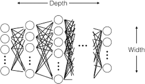
The way we approach dimensioning at RAM is “constructive” in the sense that we tend to start with simple and small artificial neural networks, and then increase width and depth incrementally until we find what seems to be an optimal network size. Given the size of our datasets, the largest which is typically dozens of GB with millions of single stock observation periods, we never reach the thousands of layers found in some of the most recent image recognition deep neural networks.
“ The more data we have in our training and validation samples, the more parameters the algorithm can handle without overfitting and loss of generalization. ”
In the case of an artificial neural network, dimension both represents the width and the depth (number of layers) of a neural network. When one scales up a network from low dimensions, it is either possible to increase the width or the depth of the network. There is solid theoretical foundations for the strong performance of deep networks.
Montufar, Pascanu, Cho and Bengio (2014) demonstrate the strength of a combination of layers to capture complexity, identifying a number of input regions exponential to the depth of the network. 1
In practice however it does seem that deep learning practitioners tend to exaggerate the number of layers in their networks, sometimes massively over-dimensioning them, while much smaller wider alternatives would both improve accuracy and save them computing costs, see for instance Wide Residual Networks by Zagoruyko & Komodakis, 2016. 2
Schmidhuber, Greff and Srivastava also published a very interesting article aiming to overcome the difficulty and limits of very-deep neural network training (up to close to arbitrary size) in their Highway Networks (2015). 3
1 Reference: https://arxiv.org/pdf/1402.1869.pdf
2 Reference: https://arxiv.org/pdf/1605.07146.pdf
3 Reference: https://arxiv.org/pdf/1505.00387.pdf
PART C
When designing a machine learning model, it is crucial to consider how well the model can generalize to new data. If the model is appropriately fitted, it will be able to make predictions based on data it has never seen before.
If the model is under or over fitted, generalization won’t be possible. The control of the fit is based on the bias-variance tradeoff.
As illustrated below, high bias is a characteristic of an underfitted model and high variance is a characteristic of an overfitted model.
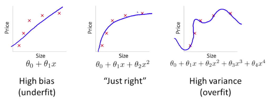
Image source : i.stack.imgur.com/t0zit.png
How to control the generalization
To control the generalization of the model, we analyze the convergence of the loss function over training and validation samples. A loss function is a measure of how well the algorithm models the given data.
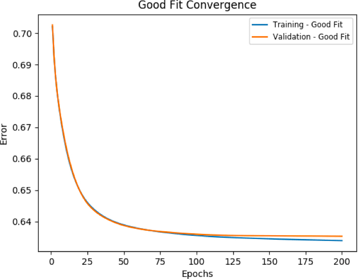
Good Fit
Ideally, the situation when the loss function reaches a global minimum, the model is said to have a good fit on the data. This case is achievable at the point between overfitting and underfitting. With the passage of time, our model will keep on learning and will be able to generalize. As such, the error for the model on the training and the validation data will keep on decreasing.
Under Fit
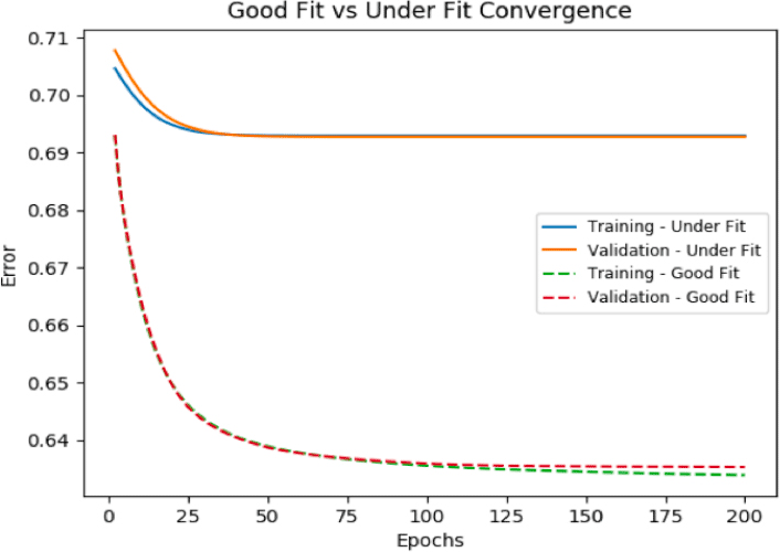
Models with a high bias will not learn enough from the training data and will oversimplify the model. Consequently, it cannot capture the underlying trend of the data. As observed on the chart below, this leads to a high error count on both the training and validation data.
Over Fit
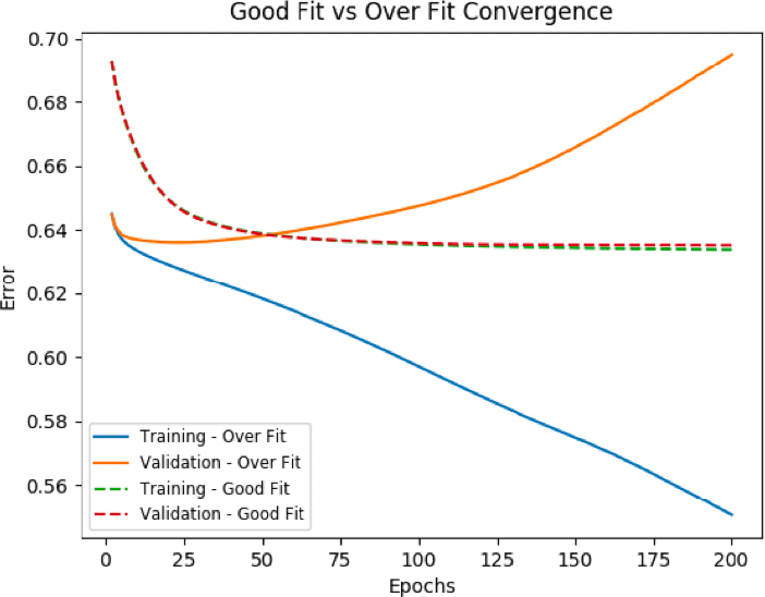
Models with high variance overlearns on the training data, capturing all its specificities (including true properties but also noise), and does not generalize on new data. As a result, such models get opposite convergence patterns on training and validation loss function: the more the model learns (decrease in training error), the less it is able to generalize (increase in validation error).
How to improve the generalization
All the steps described in previous chapters are important to help the generalization of the model, including data related matters (size of the dataset, data preprocessing, features selection) and algorithm specific issues (type and dimension of the algorithm). Additionally, several techniques can be used to control the machine during the learning process, to achieve an optimal fit:
Fold cross validation
In K Fold cross validation, the data is divided into k subsets. A training/validation process is repeated k times, such that each time, one of the k subsets is used as the validation set and the other k-1 subsets are put together to form a training set. The error is defined as the averaged error over all k trials. This helps to reduce bias/ underfitting risk as most of the data is used for training and reduces variance/overfitting risk as most of the data is also being used for validation.
Regularization
One of the most common mechanisms for avoiding overfitting is called regularization. Many regularization approaches have been developed and below we are presenting two internally used techniques.
Ridge Regression:
To reduce the impact of irrelevant features on the trained model, another element is added to the loss function. This element leads to the loss function being negatively impacted by high features coefficients. As the function is minimized, the coefficients tend to be reduced, resulting in a simplified model, thus less prone to overfitting.
Loss = Σ( Ŷi– Yi)2 + λΣ β2
with
Σ( Ŷi– Yi)2 = Original Loss
λΣ β2 = Regularization term
Dropout:
Deep neural networks have many parameters and as such, are prone to overfitting. The Dropout is a technique for addressing this problem. The concept is to randomly drop units (along with their connections) from the neural network during training. This prevents units from co-adapting too much*.
*Dropout: A Simple Way to Prevent Neural Networks from Overfitting.
Nitish Srivastava, Geoffrey Hinton, Alex Krizhevsky, Ilya Sutskever, Ruslan Salakhutdinov; 15(Jun):1929−1958, 2014.
Early Stopping
During the training of the machine, there will be a point when the model will stop generalizing and start learning the statistical noise in the training dataset. A technique called Early Stopping is used to avoid overtraining by stopping the training when a trigger is reached. For instance, this trigger can be the point where the validation error starts increasing.
Learning rate
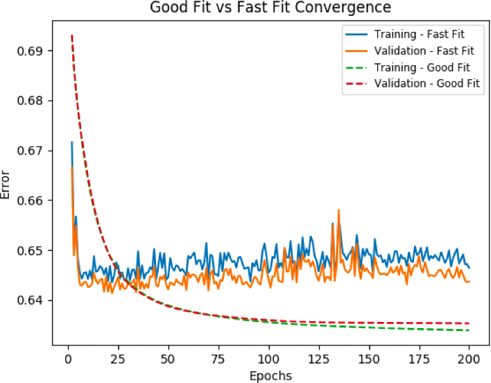
Learning rate is a hyper-parameter that controls how much we are adjusting the weights of our network following a training step. The lower the value, the lower the impact of the correction. Our approach is to avoid the risk of setting a rate that would be too high or too low by using an adaptive learning rate which evolves during this training process. While using a low learning rate might seem a good idea in terms of ensuring that we do not miss the global minimum, it could also mean that the convergence will take a long time, especially if it gets stuck on a region with the same error (plateau). An increasing learning rate helps the convergence to progress faster and allows for traversal of plateau and saddle points (critical point in which some dimensions observe a local minimum, while other dimensions observe a local maximum). However, when the learning rate is too high, huge steps will be taken and the minimum will never be reached. As observed on the chart below, the loss is reduced very quickly, but then the parameters become unstable and the loss diverge from the minimum on both training and validation set.

PART D
At RAM, we believe focusing on model interpretability is key when developing stock selection strategies which combine a high number of factors. Interpretability means understanding why a model makes a certain prediction.
It’s even more important since:
However, we are using deep learning models which are, by their very nature, complex. Complex models generally allow to obtain good predictive accuracies, which often comes at the expense of interpretability.
Different approaches can be used. The most direct ones are perturbation-based methods; they directly compute the attribution of an input feature (or set of features) by removing or altering them (adding noise for example) and running a prediction (with a simple forward pass) on the new input, measuring the difference with the original prediction. Other popular approaches include the “gradient- based” methods; they compute the attribution by calculating the partial derivatives of the prediction with respect to each input feature and multiplying them with the input itself. Other popular methods include “relevance backpropagation” and “attention-based methods”, however we will not discuss these here.
Interpretability has been an increasing area of research recently, and many packages have been proposed to enhance model explainability, such as SHAP – SHapley Additive exPlanations, which is an attempt to unify some of these attribution methods.
The SHAP unified approach to interpretability
SHAP is presented as a unified approach to interpreting model predictions, we use it to measure variable importance, and to visualize interactions between some input variables and the response variable. This approach comes from game theory and is based on Shapley values (named after game theorist and Nobel prize winner Lloyd Shapley). They are used to fairly distribute credit or value to each individual player/participant in cooperative situations, or in short, to design a fair payout scheme. In summary, Shapley values calculate the importance of a feature by comparing what a model predicts with and without the feature. However, the order in which a model sees features may have an impact on its predictions, thus this comparison is done in every possible order.
In their paper presented at NIPS 2017, Lundberg and Lee present an approach to compute “Shapley Additive exPlanations”, an additive feature importance measure, and theoretical results (derived from a proof from game theory on the fair allocation of profits). This showed that, in the class of additive feature attribution methods, their approach is the only one which verifies a number of desirable properties, in particular local accuracy (the sum of all the feature importance should sum up to the total importance of the model) and consistency (if we change a model such that it relies more on a feature, then the attributed importance for that feature should not decrease).
The SHAP package: an efficient model interpretation
The SHAP library is designed to calculate Shapley values significantly faster than if a model prediction had to be calculated for every possible combination of features, by implementing model specific algorithms, which take advantage of different model’s structures. For example, SHAP’s integration with gradient boosted decision trees takes advantage of the hierarchy in a decision tree’s features to calculate the SHAP values, in polynomial time instead of the classical exponential runtime. For Python, the SHAP package provides Shapley values calculations and (partly interactive) plots to explore Shapley values across different features and/or observations.
Feature Importance
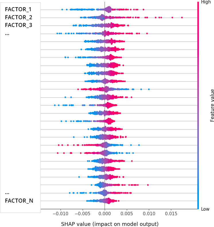
The figure below shows the distribution of Shapley values, for each feature, across the observations in a test sample used for a stock selection strategy that we’ve implemented at RAM. The most discriminative feature (factor) appears at the top of the chart. The sign shows whether the factor value moved the prediction – a measure of expected forward stock behavior – toward positive (positive SHAP) or negative (negative SHAP).
Feature Importance

The color reflects the order of magnitude of the factor values (low, medium, high). This way the plot immediately reveals that low (blue) values on the top seven factors deteriorate prospects for a given stocks.
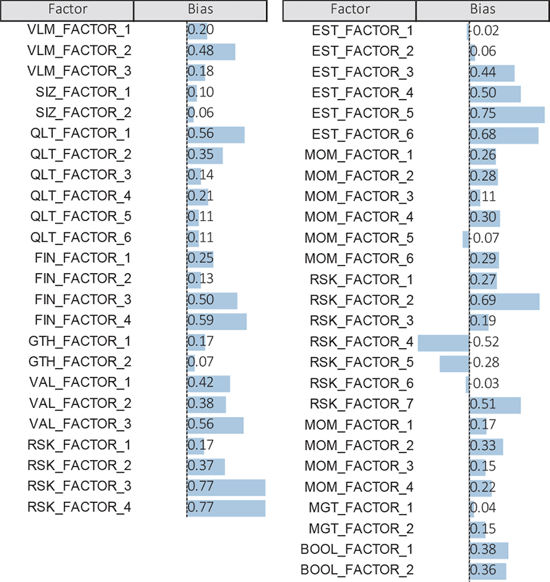
It is also important to monitor input factor biases across a stock selection.
At RAM, we also gain comfort in the predictions of our stock selection models by looking at the average factor biases for a selection at a given date. They must make sense on average and be relatively stable historically. The chart below shows an example of average factor biases for a long-only stock selection model based on 51 factors within emerging markets (the higher the better), at a given date.
Factor Biases
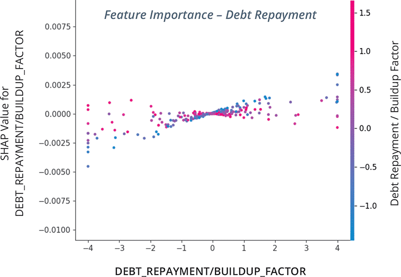
Additional interactions charts are available, such as the one below representing SHAP value for the repayment / build-up of debt in our stock selection model.
We were mentioning previously that debt levels and debt dynamics have an unclear impact on expected forward stock behavior, as their interactions with future returns are not linear. The chart below shows that although the repayment / build-up of debt has a slight positive impact on expectations on average, the model distinguishes between stocks ranking positively on a growth factor (in red) and the others (in blue) : the latter ones are clearly expected to be rewarded by the market when they are able to repay their debt, or conversely, to be punished if they accumulate excessive debt.
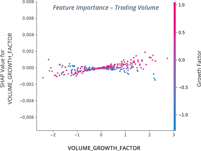
Below we present another interaction chart showing that trading volume growth has an impact on future returns after conditioning on whether a stock ranks positively on a growth factor:
The general enthusiasm for machine learning techniques will not turn out to be a short-lived fashion trend. It is proving to be, across numerous fields of application, the most efficient tool to extract information and build predictive models from large datasets.
The significant investments of tech giants into the technology and hardware supporting deep learning will help maintain this trend. The flexibility and robustness of their open-source development frameworks, as well as the significant processing power accessible (either directly or through their highly-evolutive cloud infrastructures), make machine learning techniques efficient data processing techniques. This is increasingly welcome at a time when digital data is exploding, alternative or unstructured financial datasets.
But we must be conscious that the history of artificial intelligence is awash with over-exuberant expectations.
Here, the most stunning example could be the optimistic forecast of cognitive scientist Minsky in 1970 : “In from three to eight years we will have a machine with the general intelligence of an average human being”. Who would only accurately predict today when fully autonomous self-driving cars will be reliable ?
We prefer to regard machine learning techniques as a generalization of traditional data processing techniques, and our research efforts are equally focused on testing models and controlling them by making sure they generalize and provide tangible results. At a time when the number of attempts to generate truly human-like AI is increasing and excitation about fully-autonomous vehicles is growing, we embrace initiatives about “Human trust in AI”.